Wildlife Sciences

The Art and Science of Counting Deer

Charles E. Kay. 2010. The Art and Science of Counting Deer. Muley Crazy Magazine, March/April 2010, Vol 10(2):11-18

Full text:

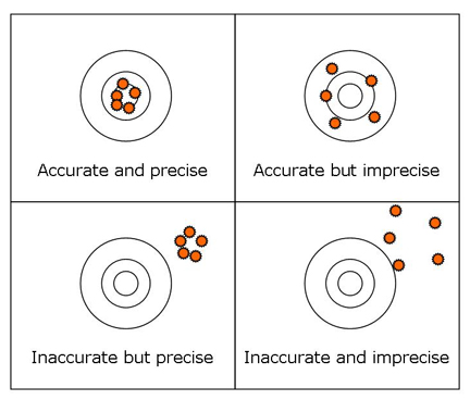
It is the simplest of questions and upon which all management is based. It is also the first thing most hunters want to know. How many deer are there? The answer? Well, there are no answers, only estimates. In addition, one needs to understand the difference between precision and accuracy. Think of precision as shooting a five-shot, half-inch group at 100 yards, but the group is 20 inches high and to the right. The shots have been very precise, almost in the same hole, but they were not accurate because they were far from the center of the target. Accuracy is hitting the bullseye. So, an estimate can be precise without being accurate. Estimates that are both precise, low variation, and accurate, close to the true number, are very difficult and very expensive to obtain. Moreover, all population estimates contain assumptions, as well as sampling errors and statistical variation.

Since the advent of modern game management, various methods have been developed to count wildlife. Entire books have been written on the subject and there are enough scientific studies to fill a small library. Here, I will discuss only the techniques that have been, or are commonly used to estimate the number of mule deer and elk on western ranges. This includes ground counts, aerial surveys, population models, pellet-group counts, and thermal imaging.

The oldest and simplest method is ground counts. As the name implies, these are simply counts conducted on foot, horseback, or from vehicles by either one or more observers. While relatively inexpensive, this method is neither precise nor accurate. There is the problem of double counting when the deer run over the hill into the next canyon that has not yet been surveyed and under counting when animals are hidden from view by vegetation or topography. Today, ground counts are seldom used to estimate herd numbers but they are still commonly employed to estimate fawn:doe ratios or buck:doe ratios under the assumption that doe, fawn, and buck sighting rates are similar, which they are not. If bucks are more difficult to see than does because of the habitat the males occupy, or their behavior, ground counts will underestimate the number of bucks.

Due to the shortcomings of ground counts, wildlife biologist were quick to take to the air, first in airplanes and later in rotary aircraft. To make a long story short, counts from helicopters are more accurate than population surveys from fixed-wings. Any aerial count, though, is subject to errors, because even from the air you do not see all members of a population, be they mule deer or elk. This is what, in the scientific literature, is known as sightability bias. Even in experiments where livestock have been placed in flat, grassy pastures, aerial observers fail to record all the animals.

Based on various studies, the proportion of the herd seen from the air varies with the speed of the aircraft — the slower you fly the more animals you see; the height of the aircraft above the ground — the lower you are, the more animals you see; the distance between flight lines — the closer together the flight lines, the more animals are seen; snow cover, as most population counts and surveys are done during winter when the animals are concentrated, the best counting conditions usually occur after a heavy, fresh snowfall; vegetative cover — as trees, or hiding cover increases, fewer animals are seen; topography — fewer animals are seen if the canyons are deep or the mountains steep; observer fatigue — as observers tire, counting efficiency declines; experience — seasoned observers see more game than novices; group size — it is easier to see animals if they are in large herds than if they are scattered; time of day — more animals are seen at first and last light than during midday, the same as when you are hunting; and the behavior of the animals, animals that are up and moving and easier to spot than ones that are bedded; among other factors.

Elk are easier to count than mule deer because when approached in a helicopter, elk herd up and typically stay together. Mule deer, on the other hand, tend to go their separate ways, which makes counting more difficult and less accurate.

Then there is the problem of politics. Does the biologist and department higher-ups want a low count or a high count? If sportsman are claiming there are no deer left, state officials would certainly like a high count. If, however, ranchers are complaining that there are too many elk, the pressure will be on for a low count. A while back I did some consulting for an wealthy oilman who had purchased a ranch in Utah’s Book Cliffs and who was engaged in a dispute with federal and state officials over how many elk were on his property. The Utah Division of Wildlife Resources (DWR) would conduct a winter helicopter count and I would sit behind the state biologist and write down how many elk we saw, when, and where. And there never was any disagreement between myself and the state on how many elk we saw.

A week or so later, after the elk had a chance to settle down, I conducted my own count using one of the billionaire’s helicopters and surprise, surprise, I saw more elk than the state claimed were in the entire herd. Why the difference? First, for whatever reason, we began our private counts an hour earlier than the state started its surveys. That put us in the counting area right when the sun first came up, unlike DWR. Next, after learning which areas the elk favored, I flew those drainages first. Thus, I flew the bottom of Bitter Creek at first light, and we counted and video-ed 1,200 elk. When the state did its counts, either by accident or design, they flew the bottom of Bitter Creek at two or three in the afternoon and saw a lot fewer elk. This happened in other elk concentration areas, as well.

So you do a helicopter count, or you fly with your state biologist when he or she does a survey, and you see (let’s say) 2,000 mule deer. What does that mean? Absolutely nothing except that you saw 2,000 deer, because you have no way of knowing whether that number is precise or accurate. The only way to determine what the 2,000 figure means is to do additional counts, so that statistically you can develop a mean and a measure of the variation around that mean, which is usually expressed as the standard deviation.

Assume that you have counted your local mule deer herd multiple times and can now calculate a mean of 2,000 + or - 500 deer (the plus or minus being the standard deviation). What does that mean? It means that there is a 66% probability that the actual number of deer is between 1,500 and 2,500 deer and that there is a 96% chance that the true population is between 1,000 and 3,000 deer. And this after you have spent tens of thousands of dollars doing multiple helicopter surveys. If you want more precision, say a standard deviation of only + 250 animals, that requires still more counts. But after all that, is the count accurate? Not unless you also have data on sightability.

Most sightability work in the West has been done on elk with only a few studies on mule deer, but the principles are the same. You start by marking a number of animals at random throughout the population — most such studies mark only females. Today, this is usually done by net-gunning the deer and attaching a highly-visible radio collar. Now that you have say 100 marked mule deer. Next you conduct a helicopter count, and for sake of discussion assume that you see 2,000 deer, only 50 of which are marked. In this example, you have seen 50% of the marked animals, which you can then use to correct your raw count for sightability bias. This produces a population estimate of 4,000 deer, which is more accurate than survey counts alone but which still lacks a mean and standard deviation. Hence, additional counts and sightability estimates are needed to develop a measure that is both precise and accurate.

Repeated counts using marked animals are termed a Lincoln or Peterson Index and involve various assumptions. The most important assumption is that the marked animals are randomly distributed throughout the population and that all the marked animals are in the area being counted. This is where the radio collars are critical. Immediately after the helicopter count is completed, you over-fly the area in a fixed-wing and radio-relocate all the marked deer to be sure that the animals are actually in the study area. If some of the marked deer were not in the counting area, then you have to adjust your sightability estimate by the appropriate percentage. If the marked animals are clumped, which you can tell by the radio relocations, you have to mark additional animals, where none presently exist, before repeating the count.

When state biologist conduct game surveys, they always claim they are doing the counts under similar circumstances — the same snow conditions, weather, and the like. The available data, however, do not support that assumption. In one New Mexico study, repeated helicopter counts found that the sightability of marked elk varied from 19% to 69% and averaged 50%. The work that has been done with mule deer has reported similar results. Sightability varies widely and averages only around 50% on winter ranges with some vegetative cover. Which is why single counts, or trend counts, without marked animals are always suspect. Moreover, most game departments only have enough resources to do simple counts, without marked animals, in any one herd unit, only once every few years.

Because of the difficulties, as well as the expense of producing accurate counts, especially for mule deer, many game departments have turned to population models. In my home state of Utah, DWR counts elk in herd units once every three years, with no sightability estimates, and does not count mule deer at all. Instead they, like other game departments, use a computer program called POP II to estimate mule deer numbers. There are difficulties with using any population model, though, as all are subject to errors and political abuse. That is to say, you can produce any number you want by manipulating the variables in POP II. The other problem is that the public, including hunters, have little understanding of population models and tend to believe whatever comes out of a computer, which is a serious error.

POP II is a Leslie Matrix type model that today can be run on most home computers using a spreadsheet. POP II is as basic as it gets, and for our purposes and most game department applications, we need be concerned mainly with the female segment of the herd. First, you need an estimate of how many yearling does are added to the population each year — this can be determined in a number of ways, many of which are time consuming and expensive. Next you need an estimate of adult female survival or mortality — survival being the inverse of mortality. If survived is 85%, mortality is 15%. Thus, if you have a 1,000 one-year-old deer and mortality is 15%, you also have 850 deer in the second, or two-year-old age class and so on for each succeeding year until the last of the starting deer is dead. The male segment of the population is treated the same way on a different part of the spreadsheet, or on a different spreadsheet. You can then tinker with the model by changing input variables and observing how the computer-generated population responds.

This is usually done by changing either fawn of adult female survival and is called a sensitivity analysis. Research has shown that the most important variable in population growth or decline is adult female survival, not fawn production or survival. If you have high adult female survival, your deer herd can maintain its numbers even if there is a poor fawn crop. And conversely, if you have low adult female survival, high fawn survival will not save your herd. By changing male mortality in the male portion of the population model, you can also estimate how many bucks there will be in various age classes under different harvest regimes. So far so good. Difficulties arise, however, when you look at how the input variables are determined, as well as their underlying assumptions. This is true of all models, be they for deer herds or climate change.

The most obvious problem is how was the starting population determined? As you might imagine, you get a completely different model-derived deer population in future years if you start with 10,000 deer instead of 5,000 deer in year one. So again, the first question the informed sportsman or woman needs to ask is how was the initial population number obtained? A single ground count? Multiple aerial counts? Or did someone just guess? Too often, the latter is the case.

Next, how do you estimate adult female mortality? You start by capturing a large number of animals and fitting them with radio collars that contain a mortality switch, which changes signal rate if the collar has not moved in 12 hours. If the collar is not moving, the animal is assumed to be dead. Having done all this, which is exceedingly costly in and of itself, you then have to fly at least once a month to check on every collared animal. If you obtain a mortality signal, you then have to go in on the ground and find the dead deer. In addition, you need to do this every month for 12 months before you get a single data point or estimate.

Moreover, in studies where this has been done, mortality differs not only from age class to age class, but also from year to year, and from area to area within a given year. Therefore generic survival estimates are always questionable. Finally, male mortality is generally not estimated this way due to the much higher cost; i.e., because bucks are killed by hunters, many more bucks need to be radio-collared, compared to unhunted does, to maintain an adequate sample size. Instead, male mortality is generally estimated by less accurate methods.

What this all means is that to run POP II correctly you need much more data than if you did repeated counts with marked animals. Plus, each of the mortality terms includes statistical variation that is seldom measured and never included in the model’s calculations. It is the old story of poor data in and even worse “data” out. Hence, if your state fish and game department uses POP II, or any other population model to estimate mule deer numbers, be forewarned. Do you want a low population estimate? Or a high population estimate? Do you want a declining population? Or an increasing population? You can get whatever answer you want by varying the input parameters.

In the Book Cliffs elk dispute that I mention earlier, DWR used POP II to determine how many cow elk permits had to be issued to hold the elk herd constant. The rancher’s attorney was able to get a copy of the POP II input/output used by the state. When I checked the numbers, I found that they had used an adult female survival rate that was lower than the calf survival rate they had employed. This was an immediate red flag because of all the ungulate studies that have been done around the globe, none has reported an adult female survival rate lower than calf or fawn survival.

The rancher’s attorney pointed this error out to the Wildlife Board, which is supposed to oversee DWR, but the Wildlife Board ignored our analysis even though we had retained a world-class modeling expert. The state wanted to kill as few cow elk as possible and they manipulated the model until they got the result they wanted. That is to say, if natural mortality is assumed to be high, as in this case, fewer cow elk have to be shot to hold the elk herd constant. Interestingly, DWR had no actual data on cow elk mortality in the Book Cliffs or anywhere else in Utah.

To overcome the problems of daylight aerial counting and population models, a few researchers have experimented with forward-looking infrared or thermal imaging. All mammals give off heat and by measuring the difference in the heat given off by various objects, you can create a thermal picture or image. This is usually done at night, after the rocks and soil have given off the heat of the day. This is different than night vision, which magnifies the available light. Thermal imaging measures heat. This is what the U.S. military uses to shoot up the bad guys on dark nights in Iraq and Afghanistan. The problem is that the publicly available technology cannot see, or measure heat, through vegetation and thus is no more useful than visual counts. The hope is that someday the military will declassify the good stuff and we will be able to count every deer in a herd from 150 miles up in space.

I have already outlined the difficulties of counting deer or other animals from the air due to the hiding cover provided by thick vegetation or rough topography. In southeast Alaska the conditions are so difficult, lots of tall trees and steep mountains, that the Alaska Department of Fish and Game uses a very old method to estimate blacktailed deer numbers — pellet group counts. I assume we all know what a pellet group looks like, but do you know how many times a deer defecates per day? Well, biologists have figured that out.

To use this method you first count the number of deer pellet groups on plots of known area in different vegetation types. You then divide those data by the deer defecation rate to obtain deer use days per acre by vegetation type. Next you estimate the area of each vegetation type in the herd unit. Then you multiply deer use days per acre by the acreage of each vegetation type, sum, and divide by 365 to obtain a deer population estimate. A long way to go with lots of sampling error. This technique is also used by Arizona to estimate the number of mule deer in the famous Kaibab herd. The vegetation, tall shrubs and pinion-juniper, is so thick on the herd’s winter range and the canyons so deep that aerial counts simply do not work on the Kaibab.

This discussion has turned out to be a lot longer than the editor of Muley Crazy would have liked, but as you have seen, counting deer and estimating deer populations is very complicated — and remember I have only hit the high points and avoided most of the statistics. For instance, I have discussed only total counts, not partial counts. In a randomized block or strip design, you only count a small percentage of the total area and then multiply that density estimate by the size of the entire study area to obtain a population estimate, which introduces even more potential error. The same is true with a stratified block or strip design.

The lesson, though, is that any mule deer population numbers your game department produces are all estimates, with both sampling error and statistical variation even if the latter are never mention, which is most often the case. But now at least you know what questions to ask your local biologist to determine if his or her estimates are precise and accurate, or simply guesses. Humans guess all the time. We call it gambling. Do you want to gamble with our mule deer herds? As you might guess, I think that would be a serious error.